跟着顶刊学分析之偏最小二乘路径建模

偏最小二乘路径建模 (PLS-PM) 是一种结构方程建模方法,主要用于分析具有复杂因果关系的多变量数据,特别是在处理潜在变量(无法直接观测但可以通过其他可观测变量来间接反映的变量)之间的关系时非常有用。它允许研究观测变量(observed variables)和潜变量(latent variable)之间复杂多元关系的统计方法。
10.1038/s41467-024-53753-w (Fig.3)
这个示例根据The biogeography of soil microbiome potential growth rates,这篇文献整理而来。通过PLS-PM方法分析了土壤微生物组潜在生长率的数据,探索了环境因素、土壤特性、微生物特性和群落结构对生长率的影响。代码的主要步骤包括数据加载、变量选择、数据预处理(对数变换和标准化)、模型定义(块和路径)、模型拟合以及结果分析。每个步骤都基于研究的科学假设和统计分析的需求,确保了模型的准确性和可解释性。
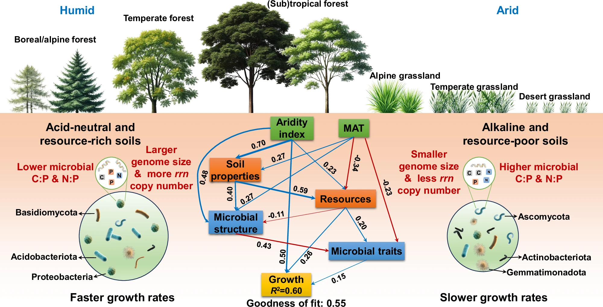
The partial least squares path model depicts factors influencing microbial potential growth rates through direct and indirect pathways. Blue and red arrows indicate positive and negative effects, respectively, while the indicated values on the arrows are the path coefficients for the inner model. The path coefficients for outer models of the partial least squares path modeling are shown in Supplementary Table 1. C is carbon, N is nitrogen, and P is phosphorus. The soil microbiome in acid-neutral soils with high organic matter and nutrients (resource-rich) in humid regions, dominated by Basidiomycota, Acidobacteriota, and Proteobacteria, exhibits a large genome size and low biomass C:P and N:P ratios, indicating a high potential growth rate. Conversely, in resource-poor, dry, and hypersaline soils, the microbiome, dominated by Ascomycota, Actinobacteriota, and Gemmatimonadota, displays a lower potential growth rate, suggesting that resource acquisition and stress tolerance tradeoff with growth rate. Source data are provided as a Source Data file.
关键要点
- 研究背景:研究通过偏最小二乘路径建模(PLS-PM)分析土壤微生物组潜在生长率(Gmass)的生物地理分布,揭示环境因素、土壤资源、微生物群落结构及其特性如何通过直接和间接路径影响生长率
- 核心发现:微生物群落结构通过改变微生物特性(基因组大小、核糖体 RNA 拷贝数、最适温度、生物量化学计量)间接影响潜在生长率,而非直接作用。基因组大小是关键的生命历史特性,影响微生物丰度、生长率和代谢能力
- 环境与生长率关系:资源丰富、酸中性、湿润地区的土壤微生物组(以 Basidiomycota、Acidobacteriota 和 Proteobacteria 主导)具有较大基因组大小和较低的生物量 C:P 和 N:P 比,表现出高潜在生长率;而资源匮乏、干旱、高盐土壤(以 Ascomycota、Actinobacteriota 和 Gemmatimonadota 主导)则生长率较低,反映资源获取和应激耐受性与生长率的权衡
偏最小二乘路径建模
加载包和数据
1 | # https://www.nature.com/articles/s41467-024-53753-w |
这些列代表了土壤微生物组生长率分析中所需的关键变量,包括:
- 微生物特性:MBCtoP(微生物生物量碳与磷的比值)、MBNtoP(微生物生物量氮与磷的比值)、F_genome_size(真菌基因组大小)、B_genome_size(细菌基因组大小)、optimum_tmp(最适生长温度)、rrn_copy_number(核糖体 RNA 运转数)
- 环境因素:AI(干燥指数)、MAT(年平均温度)、pH(土壤 pH 值)、CS(可能为黏土含量或土壤结构)
- 土壤资源:SOC(土壤有机碳)、TN(总氮)、TP(总磷)、DOC(溶解有机碳)、AvaiN(可用氮)
- 微生物群落结构:Ascomycota、Actinobacteriota、Gemmatimonadota、Acidobacteriota、Proteobacteria、Basidiomycota(这些是微生物门水平的相对丰度)
- 变量:RelGrowth(相对生长率)
这些变量的选择基于研究的目标,即探索环境因素、土壤特性、微生物特性和群落结构如何影响土壤微生物组的生长率。
1 | # 查看数据 |
数据处理
1 | # 对数变换 |
定义潜在变量块
1 | # 定义潜在变量块 |
定义路径矩阵
1 | # 定义路径矩阵 |
1 表示有从列块到行块的路径(即列块影响行块); 0 表示没有路径。
路径矩阵反映了研究的假设,即环境因素影响土壤特性和资源,进而影响微生物群落结构和特性,最终影响生长率。
拟合 PLS-PM 模型
1 | # 拟合 PLS-PM 模型 |
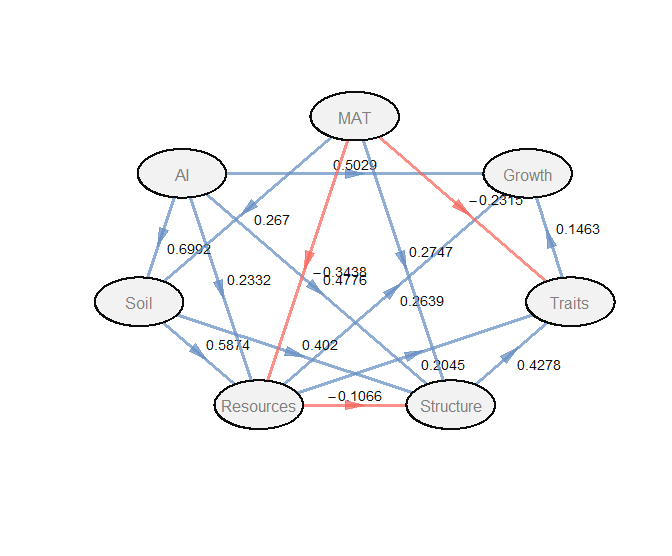
生成路径图,查看因果关系的路径图
1 | # 生成路径图,查看因果关系的路径图 |
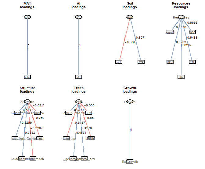
生成外模型图
1 | # 生成外模型图 |
综合结论总结
- 微生物群落结构对潜在生长率的影响路径:PLS-PM 模型表明,微生物群落结构(由主要真菌和细菌门类组成,如 Ascomycota、Basidiomycota、Actinobacteriota 等)通过调节微生物特性(Traits 块,包括基因组大小、rrn 拷贝数、最适温度、生物量化学计量)间接影响潜在生长率(Gmass)。模型中,Structure 到 Traits 的路径系数为 0.428(p < 0.001),Traits 到 Growth 的路径系数为 0.146(p < 0.001),而 Structure 到 Growth 的直接路径不显著(被移除)。这表明微生物群落组成通过塑造功能特性(如代谢能力和生长潜力)间接调控生长率,而非直接决定生长率。这种间接作用强调了微生物生态系统中群落结构与功能特性之间的复杂相互作用
- 基因组大小的关键作用:真菌和细菌基因组大小(F_genome_size 和 B_genome_size)对潜在生长率有正向影响(外模型载荷分别为 0.498 和 0.463),表明较大基因组具有更广泛的代谢能力,支持更高的生长潜力
- 统计显著性:大多数路径系数高度显著(p < 0.001),如 AI -> Growth、Resources -> Growth 和 Structure -> Traits,验证了模型路径的稳健性
- 模型拟合度:PLS-PM 模型的总体良好度(Goodness-of-Fit, GoF)为 0.5503,低于理想值 0.7,但仍表明模型具有一定的解释力
代码简洁版
1 | # 加载所需要的包 |
版本信息
1 | sessionInfo() |
- Titre: 跟着顶刊学分析之偏最小二乘路径建模
- Auteur: Xing Abao
- Créé à : 2025-04-24 10:00:00
- Mis à jour à : 2025-10-22 12:15:26
- Lien: https://bioinformatics.vip/2025/04/24/SCI/250424_sci_partial_least_squares_path_model/
- Licence: Cette œuvre est sous licence CC BY-NC-SA 4.0.