跟着顶刊学分析之随机森林

Xing Abao Lv3

本示例参考Prophage-encoded antibiotic resistance genes are enriched in human-impacted environments

随机森林是一种强大的数据挖掘工具,能够处理高维度、多变量且复杂相关的数据,在本研究中帮助揭示了哪些人类相关活动(如抗生素使用、经济发展、农业生产等)最能解释`ARGs`在不同环境中的分布差异。这篇发表在 Nature Communications 的文章,通过结合大规模多组学数据与随机森林建模,不仅深化了我们对噬菌体在抗生素耐药性扩散中作用的理解,也为全球抗生素耐药风险的评估和干预提供了新的视角和工具。结果显示,人类活动显著促进了前噬菌体携带耐药基因的富集,这些基因不仅数量更多,而且更容易在不同生态系统间转移和表达。进一步的实验证明,这些由前噬菌体携带的耐药基因可以实际赋予宿主细菌抗药性。

随机森林建模

加载包和数据

1
2
3
4
5
6
7
8
9
# 加载所需要的包
suppressMessages(suppressWarnings(library(rfPermute)))
suppressMessages(suppressWarnings(library(randomForest)))
suppressMessages(suppressWarnings(library(ggplot2)))
suppressMessages(suppressWarnings(library(RColorBrewer)))
suppressMessages(suppressWarnings(library(A3)))

# 数据加载
data_pca = read.delim("data/HH.bacteria_ARG_RF.txt", sep = "\t", header = TRUE)

读取数据文件,包含细菌 ARGs 数据和 13 个环境或微生物群落特征。

查看数据

1
2
3
4
5
6
7
8
9
10
11
12
13
14
15
16
# 查看数据
head(data_pca)
## Land.Use.and.Land.Cover.Change Anthropogenic.biomes.of.the.world Clinical.Antibiotic.Usage Pesticide Energy.Extraction.and.Production Agricultural.Crops Forage.Crops
## 1 -0.008558508 0.0449743245 -0.03750679 -3.095344e-02 -0.050770707 -0.017596450 0.0745902209
## 2 0.033989202 -0.0007879086 -0.03501022 -2.086723e-02 -0.022458302 0.069431652 -0.0050333596
## 3 0.032429221 -0.0036439490 -0.03459265 -1.953166e-02 -0.020598446 0.063097974 -0.0048592110
## 4 0.028703800 -0.0033364393 -0.03263086 -1.647544e-02 -0.020120168 0.056062210 -0.0055928166
## 5 -0.005187596 -0.0137431232 -0.03130477 1.550494e-03 -0.001458610 0.003901025 -0.0008462444
## 6 0.023463634 -0.0220589799 -0.04257330 -3.528928e-05 -0.003313329 -0.010207201 -0.0017533765
## Mining.and.sewage.treatment Hydraulic.Engineering Veterinary.Antibiotics Global.coal.mining.industry GDP PM2.5 HH.ARG
## 1 -0.06863079 -0.017849256 0.01421391 0.003036817 -0.005415194 0.002743616 517608.6
## 2 0.02937325 0.008129795 -0.02671757 0.028700126 0.030087984 -0.011652020 782633.2
## 3 0.02840738 0.009198630 -0.02653649 0.027335597 0.027214965 -0.012959870 807482.0
## 4 0.02885892 0.006040318 -0.01574640 0.023150146 0.019394054 -0.014715967 583647.8
## 5 0.01778400 -0.009463949 0.01067881 -0.009176268 -0.026323620 -0.006677295 0.0
## 6 0.04272488 0.019752009 0.01426311 -0.022634269 -0.004662922 -0.007297746 572947.0

数据包括相应变量HH.ARG;预测变量为前 13 个环境或微生物群落特征。

数据拆分

1
2
3
4
5
# 设置随机种子,用于重复
set.seed(123)
sample_indices = sample(1:nrow(data_pca), nrow(data_pca) * 0.3)
test_data = data_pca[sample_indices, ] # 测试集(30%)
train_data = data_pca[-sample_indices, ] # 训练集(70%)

随机抽取 30% 的行作为测试集(Test Data),剩余 70% 作为训练集(Train Data)。

将数据分为训练和测试集,用于模型训练和性能评估。

随机森林建模

1
2
3
4
5
6
7
8
9
10
11
12
13
14
15
16
# Random forest modeling using the first 13 principal components to predict HH.ARG
# 原文代码好像有问题,并没有 nrep 参数,设置了 nrep = 1000 应该是不会生效的~,只有 nPerm 参数,应该是 nPerm = 1000(不知道是不是版本问题)
# 查看了整个包的源代码,的确没有看到 nrep 参数的存在,如果有知道的小伙伴请在下面留言告知一下
# nPerm 可以设置的大一些,例如 1000;这里为了快速演示,设置为 1
rf_model = randomForest(HH.ARG ~ ., ntree = 500, data = train_data, importance = TRUE, nPerm = 1)

rf_model
##
## Call:
## randomForest(formula = HH.ARG ~ ., data = train_data, ntree = 500, importance = TRUE, nPerm = 1)
## Type of random forest: regression
## Number of trees: 500
## No. of variables tried at each split: 4
##
## Mean of squared residuals: 22837048700
## % Var explained: 75.22

建立模型预测 HH.ARG,并准备评估变量重要性。

说明

  • 使用 randomForest 包构建随机森林回归模型
  • 相应变量: HH.ARG
  • 预测变量: 训练集中除 HH.ARG 外的所有列
  • ntree = 500: 构建 500 棵决策树
  • importance = TRUE: 计算变量重要性
  • nPerm = 1: 置换检验的重复次数

nPerm

`nPerm`作用是在指定在评估变量重要性时,对每棵树的 OOB(Out-of-Bag)数据 进行置换的次数(仅用于回归问题,分类问题时候不支持)。默认值`nPerm = 1`,表示每次只进行一次置换。当`nPerm > 1`时,每次计算变量重要性时会多次置换 OOB 数据,取平均结果,从而提供更稳定的重要性估计。但置换次数并不是越高越好,增加 nPerm 会提高计算成本,但对结果的稳定性提升有限,次数差不多就行,例如 1000 此;同时仅影响重要性计算,不影响模型的预测或拟合。

模型预测和性能评估

评估模型在测试集上的预测性能。

1
2
3
4
5
6
7
8
9
10
11
12
13
14
# Predictions
predictions = predict(rf_model, newdata = test_data)

# Evaluate model performance
mse = mean((predictions - test_data$HH.ARG)^2)
r_squared = 1 - mse / var(test_data$HH.ARG)

# 均方误差(MSE)
print(paste("Mean Squared Error (MSE): ", mse))
## [1] "Mean Squared Error (MSE): 39399107632.3641"

# 解释方差(R²)
print(paste("R-squared (R^2): ", r_squared))
## [1] "R-squared (R^2): 0.69171159831207"

MSE(均方误差):预测值与实际值差的平方平均,值越小表示模型越准确。

R²(决定系数):1 - MSE / 方差,表示模型解释的变异比例,值接近 1 表示模型拟合好。

因子显著性分析(置换检验)

1
2
3
4
5
6
7
8
9
10
11
12
13
14
15
16
17
18
# Use the rfPermut() function to re-perform random forest analysis on the above data
# num.rep 可以设置的大一些,例如 1000;这里为了快速演示,设置为 1
set.seed(123)
factor_rfP = rfPermute(HH.ARG ~ ., data = data_pca, importance = TRUE, ntree = 500, num.rep = 1, num.cores = 6)

factor_rfP
## An rfPermute model
##
## Type of random forest: regression
## Number of trees: 500
## No. of variables tried at each split: 4
## No. of permutation replicates: 1
## Start time: 2025-05-08 00:51:39
## End time: 2025-05-08 00:51:45
## Run time: 6.11 secs
##
## Mean of squared residuals: 2.27e+10
## % Var explained: 78

使用`rfPermute`包进行置换检验,评估预测变量的重要性显著性。

HH.ARG ~ . 与之前模型相同,使用所有预测变量预测 HH.ARG

提取重要性分数

1
2
3
4
5
6
7
8
9
10
11
12
13
14
15
16
17
18
19
20
21
22
23
24
25
26
27
28
29
30
31
32
33
34
35
# Extract importance scores of predictive variables
importance_factor.scale = data.frame(importance(factor_rfP, scale = TRUE), check.names = FALSE)
importance_factor.scale
## %IncMSE %IncMSE.pval IncNodePurity IncNodePurity.pval
## Veterinary.Antibiotics 69.02466 0.5 4.631804e+13 0.5
## GDP 36.71122 0.5 1.283392e+13 0.5
## Hydraulic.Engineering 35.89910 0.5 1.391980e+13 0.5
## Clinical.Antibiotic.Usage 21.47663 0.5 7.828127e+12 1.0
## Pesticide 20.88377 0.5 5.545666e+12 1.0
## PM2.5 20.52189 0.5 4.045383e+12 1.0
## Energy.Extraction.and.Production 20.48274 0.5 4.867682e+12 1.0
## Anthropogenic.biomes.of.the.world 20.06789 0.5 7.357752e+12 1.0
## Global.coal.mining.industry 19.83123 0.5 5.589486e+12 1.0
## Mining.and.sewage.treatment 19.29399 0.5 6.573337e+12 1.0
## Agricultural.Crops 16.02678 0.5 4.635201e+12 1.0
## Forage.Crops 14.88528 0.5 4.449917e+12 1.0
## Land.Use.and.Land.Cover.Change 12.28250 0.5 5.240298e+12 1.0

# Extract the significance of importance scores of predictive variables
importance_factor.scale.pval = (factor_rfP$pval)[ , , 2]
importance_factor.scale.pval
## %IncMSE IncNodePurity
## Land.Use.and.Land.Cover.Change 0.5 1.0
## Anthropogenic.biomes.of.the.world 0.5 1.0
## Clinical.Antibiotic.Usage 0.5 1.0
## Pesticide 0.5 1.0
## Energy.Extraction.and.Production 0.5 1.0
## Agricultural.Crops 0.5 1.0
## Forage.Crops 0.5 1.0
## Mining.and.sewage.treatment 0.5 1.0
## Hydraulic.Engineering 0.5 0.5
## Veterinary.Antibiotics 0.5 0.5
## Global.coal.mining.industry 0.5 1.0
## GDP 0.5 0.5
## PM2.5 0.5 1.0

提取变量重要性分数,并进行标准化(scale = TRUE),量化每个主成分对模型的贡献及其统计显著性。

按重要性排序

1
2
3
4
5
6
7
8
9
10
11
12
13
14
15
16
17
# Sort predictive variables by importance scores, e.g., by "%IncMSE"
importance_factor.scale = importance_factor.scale[order(importance_factor.scale$'%IncMSE', decreasing = TRUE), ]
importance_factor.scale
## %IncMSE %IncMSE.pval IncNodePurity IncNodePurity.pval
## Veterinary.Antibiotics 69.02466 0.5 4.631804e+13 0.5
## GDP 36.71122 0.5 1.283392e+13 0.5
## Hydraulic.Engineering 35.89910 0.5 1.391980e+13 0.5
## Clinical.Antibiotic.Usage 21.47663 0.5 7.828127e+12 1.0
## Pesticide 20.88377 0.5 5.545666e+12 1.0
## PM2.5 20.52189 0.5 4.045383e+12 1.0
## Energy.Extraction.and.Production 20.48274 0.5 4.867682e+12 1.0
## Anthropogenic.biomes.of.the.world 20.06789 0.5 7.357752e+12 1.0
## Global.coal.mining.industry 19.83123 0.5 5.589486e+12 1.0
## Mining.and.sewage.treatment 19.29399 0.5 6.573337e+12 1.0
## Agricultural.Crops 16.02678 0.5 4.635201e+12 1.0
## Forage.Crops 14.88528 0.5 4.449917e+12 1.0
## Land.Use.and.Land.Cover.Change 12.28250 0.5 5.240298e+12 1.0

按`%IncMSE`降序排序重要性数据框,优先展示最重要的变量,便于可视化时突出关键预测变量。

绘制重要性柱状图

1
2
3
4
5
6
7
8
9
10
11
12
13
14
15
16
17
18
19
20
21
22
23
24
25
26
27
28
29
30
31
# Plotting the %IncMSE values of predictive variables
importance_factor.scale$OTU_name = rownames(importance_factor.scale)
importance_factor.scale$OTU_name = factor(importance_factor.scale$OTU_name, levels = importance_factor.scale$OTU_name)

gg = ggplot() +
geom_col(
data = importance_factor.scale,
aes(x = reorder(OTU_name, `%IncMSE`), y = `%IncMSE`, fill = `%IncMSE`),
colour = 'black',
width = 0.8
) +
# 横向柱状图
coord_flip() +
# 颜色渐变
scale_fill_gradientn(
colors = c(
low = brewer.pal(5, "Blues")[2],
mid = brewer.pal(5, "YlGnBu")[1],
high = brewer.pal(6, "OrRd")[4]
),
values = scales::rescale(c(0, 15, 50)),
guide = FALSE,
aesthetics = "fill"
) +
labs(title = NULL, x = NULL, y = 'Increase in MSE (%)', fill = NULL) +
theme_test() +
theme(panel.grid = element_blank(), panel.background = element_blank(), axis.line = element_line(colour = 'black')) +
theme(axis.text.x = element_text(angle = 90, hjust = 1)) +
scale_y_continuous(expand = c(0, 0), limit = c(0, 78))

gg


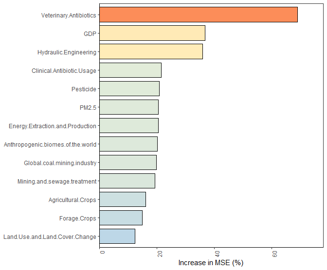
可视化主成分对模型的重要性,直观展示哪些变量对预测HH.ARG贡献最大。

添加显著性标记

1
2
3
4
5
6
7
8
9
10
11
12
13
14
15
16
17
18
19
20
21
# Mark the significance information of predictive variables
# Default p < 0.05 as *, p < 0.01 as **, p < 0.001 as ***
for (OTU in rownames(importance_factor.scale)) {
importance_factor.scale[OTU, '%IncMSE.pval'] = importance_factor.scale.pval[OTU, '%IncMSE']
if (importance_factor.scale[OTU, '%IncMSE.pval'] >= 0.05) importance_factor.scale[OTU, '%IncMSE.sig'] = ''
else if (importance_factor.scale[OTU, '%IncMSE.pval'] >= 0.01 & importance_factor.scale[OTU, '%IncMSE.pval'] < 0.05) importance_factor.scale[OTU, '%IncMSE.sig'] = '*'
else if (importance_factor.scale[OTU, '%IncMSE.pval'] >= 0.001 & importance_factor.scale[OTU, '%IncMSE.pval'] < 0.01) importance_factor.scale[OTU, '%IncMSE.sig'] = '**'
else if (importance_factor.scale[OTU, '%IncMSE.pval'] < 0.001) importance_factor.scale[OTU, '%IncMSE.sig'] = '***'
}

gg = gg +
annotate(
"text",
x = importance_factor.scale$OTU_name,
y = importance_factor.scale$`%IncMSE`,
label = sprintf("%.2f%% %s", importance_factor.scale$`%IncMSE`, importance_factor.scale$`%IncMSE.sig`),
hjust = -0.2,
size = 3
)

gg

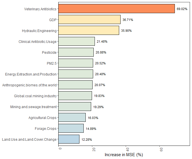
突出显著变量,帮助解读哪些主成分对模型的贡献在统计上显著。

模型整体显著性评估

1
2
3
4
5
6
7
8
9
10
11
12
13
14
15
16
17
18
19
20
21
22
23
24
25
26
27
28
29
# A3 package for evaluating model p-value
# model.fn = randomForest calls the randomForest method for computation
# p.acc = 0.001 indicates the estimation of p-value based on 1000 random permutations.
# model.args is used to pass parameters to randomForest(), so the parameters inside are based on the parameters of randomForest(). For details, see ?randomForest
# p.acc: 通过 1000 次置换估计 p 值(1/0.001 = 1000),这里为了测试,设置为了 0.1
# ntree = 500,传递随机森林参数,这里为了测试,设置了 5
set.seed(123)
factor_forest.pval = a3(HH.ARG ~ ., data = data_pca, model.fn = randomForest, p.acc = 0.1, model.args = list(importance = TRUE, ntree = 5))

factor_forest.pval
## Average Slope CV R^2 p value
## -Full Model- 73.0 % < 0.1
## (Intercept) 0 + 2.4 % < 0.1
## Land.Use.and.Land.Cover.Change 7090 + 3.4 % < 0.1
## Anthropogenic.biomes.of.the.world -41353 + 5.9 % < 0.1
## Clinical.Antibiotic.Usage 37587 - 1.9 % < 0.1
## Pesticide -22376 + 1.8 % < 0.1
## Energy.Extraction.and.Production 39878 + 2.2 % 0.1
## Agricultural.Crops -37136 + 1.0 % 0.1
## Forage.Crops 14235 + 2.7 % < 0.1
## Mining.and.sewage.treatment -27080 + 6.3 % < 0.1
## Hydraulic.Engineering 109701 + 4.9 % < 0.1
## Veterinary.Antibiotics -519640 + 21.2 % < 0.1
## Global.coal.mining.industry 33377 + 2.3 % < 0.1
## GDP 93556 + 3.8 % < 0.1
## PM2.5 28407 + 1.9 % < 0.1

model.out = as.data.frame(factor_forest.pval$table)
p.value = as.numeric(gsub("<", "", model.out[1, "p value"]))

验证模型整体是否显著(p < 0.05 表示模型预测能力超出随机水平)。

添加模型统计信息到图表

1
2
3
4
5
6
7
# Add known explanation rate of the model to the top right corner
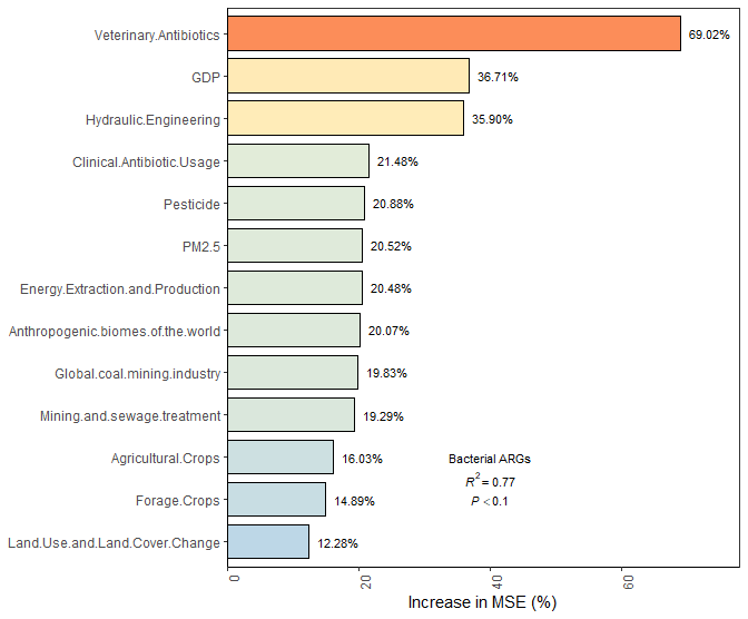
gg = gg +
annotate('text', label = 'Bacterial ARGs', x = 3, y = 40, size = 3) +
annotate('text', label = sprintf('italic(R^2) == %.2f', mean(factor_rfP[["rf"]][["rsq"]])), x = 2.5, y = 40, size = 3, parse = TRUE) +
annotate('text', label = sprintf('italic(P) < %.3f', p.value), x = 2, y = 40, size = 3, parse = TRUE)

gg

总结模型性能,增强图表的信息量。

注意事项和改进建议

但如果计算资源允许,可增加置换次数 1000 到 5000 以提高 p 值精度。

当前仅计算了测试集的 MSE 和 R²,建议添加交叉验证:

1
2
3
4
5
6
7
8
9
10
11
12
13
14
15
16
17
18
19
20
21
22
suppressMessages(suppressWarnings(library(caret)))

set.seed(123)
cv_model = train(HH.ARG ~ ., data = data_pca, method = "rf", trControl = trainControl(method = "cv", number = 5))
print(cv_model)
## Random Forest
##
## 1284 samples
## 13 predictor
##
## No pre-processing
## Resampling: Cross-Validated (5 fold)
## Summary of sample sizes: 1027, 1028, 1025, 1028, 1028
## Resampling results across tuning parameters:
##
## mtry RMSE Rsquared MAE
## 2 173379.8 0.7645675 99198.19
## 7 154867.7 0.7893561 88932.09
## 13 155936.6 0.7792823 89599.24
##
## RMSE was used to select the optimal model using the smallest value.
## The final value used for the model was mtry = 7.

总结

这段代码通过随机森林模型分析细菌 ARGs 与主成分的关系,评估模型性能,并可视化变量重要性。主要步骤包括:1. 构建和评估随机森林模型(MSE, R²);2. 通过置换检验确定主成分的显著性;3. 绘制柱状图,展示 %IncMSE 和显著性标记,添加模型统计信息。

代码简洁版

1
2
3
4
5
6
7
8
9
10
11
12
13
14
15
16
17
18
19
20
21
22
23
24
25
26
27
28
29
30
31
32
33
34
35
36
37
38
39
40
41
42
43
44
45
46
47
48
49
50
51
52
53
54
55
56
57
58
59
60
61
62
63
64
65
66
67
68
69
70
71
72
73
74
75
76
77
78
79
80
81
82
83
84
85
86
87
88
89
90
91
92
93
94
95
96
97
# 加载所需要的包
suppressMessages(suppressWarnings(library(rfPermute)))
suppressMessages(suppressWarnings(library(randomForest)))
suppressMessages(suppressWarnings(library(ggplot2)))
suppressMessages(suppressWarnings(library(RColorBrewer)))
suppressMessages(suppressWarnings(library(A3)))

# 数据加载
data_pca = read.delim("data/HH.bacteria_ARG_RF.txt", sep = "\t", header = TRUE)

# 数据拆分
set.seed(123)
sample_indices = sample(1:nrow(data_pca), nrow(data_pca) * 0.3)
test_data = data_pca[sample_indices, ] # 测试集(30%)
train_data = data_pca[-sample_indices, ] # 训练集(70%)

# 随机森林建模
rf_model = randomForest(HH.ARG ~ ., ntree = 500, data = train_data, importance = TRUE, nPerm = 1)

# 模型预测和性能评估
predictions = predict(rf_model, newdata = test_data)
mse = mean((predictions - test_data$HH.ARG)^2)
r_squared = 1 - mse / var(test_data$HH.ARG)

# 因子显著性分析(置换检验)
set.seed(123)
factor_rfP = rfPermute(HH.ARG ~ ., data = data_pca, importance = TRUE, ntree = 500, num.rep = 1, num.cores = 6)

# 提取重要性分数
importance_factor.scale = data.frame(importance(factor_rfP, scale = TRUE), check.names = FALSE)
importance_factor.scale.pval = (factor_rfP$pval)[ , , 2]

# 按重要性排序
importance_factor.scale = importance_factor.scale[order(importance_factor.scale$'%IncMSE', decreasing = TRUE), ]

# 绘制重要性柱状图
importance_factor.scale$OTU_name = rownames(importance_factor.scale)
importance_factor.scale$OTU_name = factor(importance_factor.scale$OTU_name, levels = importance_factor.scale$OTU_name)

gg = ggplot() +
geom_col(
data = importance_factor.scale,
aes(x = reorder(OTU_name, `%IncMSE`), y = `%IncMSE`, fill = `%IncMSE`),
colour = 'black',
width = 0.8
) +
# 横向柱状图
coord_flip() +
# 颜色渐变
scale_fill_gradientn(
colors = c(
low = brewer.pal(5, "Blues")[2],
mid = brewer.pal(5, "YlGnBu")[1],
high = brewer.pal(6, "OrRd")[4]
),
values = scales::rescale(c(0, 15, 50)),
guide = FALSE,
aesthetics = "fill"
) +
labs(title = NULL, x = NULL, y = 'Increase in MSE (%)', fill = NULL) +
theme_test() +
theme(panel.grid = element_blank(), panel.background = element_blank(), axis.line = element_line(colour = 'black')) +
theme(axis.text.x = element_text(angle = 90, hjust = 1)) +
scale_y_continuous(expand = c(0, 0), limit = c(0, 78))

# 添加显著性标记
for (OTU in rownames(importance_factor.scale)) {
importance_factor.scale[OTU, '%IncMSE.pval'] = importance_factor.scale.pval[OTU, '%IncMSE']
if (importance_factor.scale[OTU, '%IncMSE.pval'] >= 0.05) importance_factor.scale[OTU, '%IncMSE.sig'] = ''
else if (importance_factor.scale[OTU, '%IncMSE.pval'] >= 0.01 & importance_factor.scale[OTU, '%IncMSE.pval'] < 0.05) importance_factor.scale[OTU, '%IncMSE.sig'] = '*'
else if (importance_factor.scale[OTU, '%IncMSE.pval'] >= 0.001 & importance_factor.scale[OTU, '%IncMSE.pval'] < 0.01) importance_factor.scale[OTU, '%IncMSE.sig'] = '**'
else if (importance_factor.scale[OTU, '%IncMSE.pval'] < 0.001) importance_factor.scale[OTU, '%IncMSE.sig'] = '***'
}

gg = gg +
annotate(
"text",
x = importance_factor.scale$OTU_name,
y = importance_factor.scale$`%IncMSE`,
label = sprintf("%.2f%% %s", importance_factor.scale$`%IncMSE`, importance_factor.scale$`%IncMSE.sig`),
hjust = -0.2,
size = 3
)

# 模型整体显著性评估
set.seed(123)
factor_forest.pval = a3(HH.ARG ~ ., data = data_pca, model.fn = randomForest, p.acc = 0.1, model.args = list(importance = TRUE, ntree = 5))
model.out = as.data.frame(factor_forest.pval$table)
p.value = as.numeric(gsub("<", "", model.out[1, "p value"]))

# 添加模型统计信息到图表
gg = gg +
annotate('text', label = 'Bacterial ARGs', x = 3, y = 40, size = 3) +
annotate('text', label = sprintf('italic(R^2) == %.2f', mean(factor_rfP[["rf"]][["rsq"]])), x = 2.5, y = 40, size = 3, parse = TRUE) +
annotate('text', label = sprintf('italic(P) < %.3f', p.value), x = 2, y = 40, size = 3, parse = TRUE)

gg

版本信息

1
2
3
4
5
6
7
8
9
10
11
12
13
14
15
16
17
18
19
20
21
22
23
24
25
26
27
28
29
30
sessionInfo()
## R version 4.4.3 (2025-02-28 ucrt)
## Platform: x86_64-w64-mingw32/x64
## Running under: Windows 11 x64 (build 26100)
##
## Matrix products: default
##
##
## locale:
## [1] LC_COLLATE=Chinese (Simplified)_China.utf8 LC_CTYPE=Chinese (Simplified)_China.utf8 LC_MONETARY=Chinese (Simplified)_China.utf8 LC_NUMERIC=C
## [5] LC_TIME=Chinese (Simplified)_China.utf8
##
## time zone: Asia/Shanghai
## tzcode source: internal
##
## attached base packages:
## [1] stats graphics grDevices utils datasets methods base
##
## other attached packages:
## [1] caret_7.0-1 lattice_0.22-6 A3_1.0.0 pbapply_1.7-2 xtable_1.8-4 RColorBrewer_1.1-3 ggplot2_3.5.1 randomForest_4.7-1.2 rfPermute_2.5.4
##
## loaded via a namespace (and not attached):
## [1] gtable_0.3.6 xfun_0.51 recipes_1.3.0 vctrs_0.6.5 tools_4.4.3 generics_0.1.3 stats4_4.4.3 parallel_4.4.3 tibble_3.2.1
## [10] ModelMetrics_1.2.2.2 pkgconfig_2.0.3 Matrix_1.7-2 data.table_1.17.0 lifecycle_1.0.4 compiler_4.4.3 farver_2.1.2 stringr_1.5.1 munsell_0.5.1
## [19] codetools_0.2-20 htmltools_0.5.8.1 class_7.3-23 yaml_2.3.10 prodlim_2024.06.25 pillar_1.10.1 MASS_7.3-64 gower_1.0.2 iterators_1.0.14
## [28] rpart_4.1.24 foreach_1.5.2 nlme_3.1-167 parallelly_1.43.0 lava_1.8.1 tidyselect_1.2.1 digest_0.6.37 stringi_1.8.7 future_1.34.0
## [37] dplyr_1.1.4 reshape2_1.4.4 purrr_1.0.4 listenv_0.9.1 labeling_0.4.3 splines_4.4.3 fastmap_1.2.0 grid_4.4.3 colorspace_2.1-1
## [46] cli_3.6.4 magrittr_2.0.3 survival_3.8-3 future.apply_1.11.3 withr_3.0.2 scales_1.3.0 lubridate_1.9.4 timechange_0.3.0 rmarkdown_2.29
## [55] globals_0.16.3 nnet_7.3-20 timeDate_4041.110 evaluate_1.0.3 knitr_1.50 hardhat_1.4.1 rlang_1.1.5 Rcpp_1.0.14 glue_1.8.0
## [64] pROC_1.18.5 ipred_0.9-15 rstudioapi_0.17.1 R6_2.6.1 plyr_1.8.9 swfscMisc_1.6.6
  • Titre: 跟着顶刊学分析之随机森林
  • Auteur: Xing Abao
  • Créé à : 2025-04-27 13:22:55
  • Mis à jour à : 2025-10-22 12:15:26
  • Lien: https://bioinformatics.vip/2025/04/27/SCI/250427_sci_random_forest/
  • Licence: Cette œuvre est sous licence CC BY-NC-SA 4.0.
Commentaires