跟着顶刊学分析之非线性最小二乘法

Xing Abao Lv3

非线性最小二乘法 (Nonlinear Least Squares, NLS) 是一种常见的优化方法,用于拟合非线性模型到数据,它通过最小化观测数据与模型预测之间的残差平方和来确定模型参数的最佳值。在科学研究中,特别是在生态学、生物信息学和环境科学等领域,这种方法常用于描述复杂的非线性关系,例如物种丰度与环境变量之间的关系、病毒与宿主丰度的动态变化等。非线性最小二乘法在生态学和病毒学研究中的主要作用是帮助科学家理解和量化复杂的非线性关系,尤其是在数据呈现出非线性模式时。通过这种方法,研究者可以更准确地描述病毒与宿主、病毒与环境因子之间的动态,为揭示生态机制和生物地球化学循环提供重要支持。

R² 可以判断模型整体的拟合效果,越接近于 1,拟合效果越好;负 R² 表示模型比直接用平均值还差,拟合效果极差。

本示例参考Biodiversity of mudflat intertidal viromes along the Chinese coasts

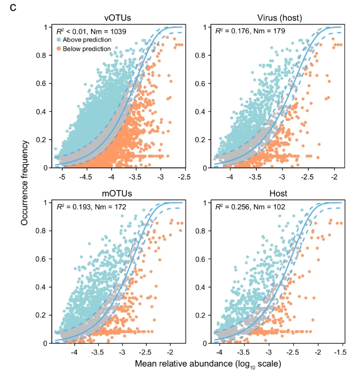
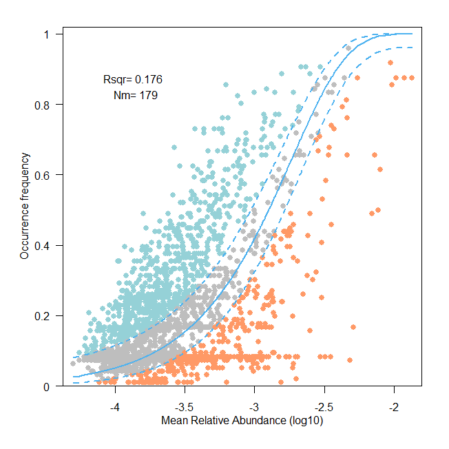
Fig.5c Neutral community model analyses based on the predicted occurrence frequencies and their relative abundances. The solid blue lines indicate the best fit to the neutral community model and the dashed blue lines represented 95% confidence intervals. Nm represents the community size times immigration, R2 represents the fit strength to this model.

R² 值小于 0.5 表明潮间带病毒群落和微生物群落的分布模式不能被中性模型(随机过程)有效解释。这支持了文章中通过多种统计方法(如 partial mantel test、variation partitioning analysis、RCbray metric 等)得出的结论,即确定性过程(如环境过滤、物种间相互作用)在群落构建中占主导地位。中性群落模型(基于随机过程的理论)无法有效解释潮间带病毒群落、原核宿主群落和微生物群落的分布模式(R² < 0.5)。这表明随机过程在这些群落构建中的作用较弱,而确定性过程(如环境选择、地理距离、病毒-宿主交互)更可能主导群落组成变异。这一结论与潮间带生态系统的复杂性和高环境异质性相符,也为文章中提出的病毒群落生态机制提供了重要支持。

非线性最小二乘法

加载包和数据

1
2
3
4
5
6
7
8
9
10
11
12
13
# 加载所需要的包
suppressMessages(suppressWarnings(library(grid)))
suppressMessages(suppressWarnings(library(glue)))
suppressMessages(suppressWarnings(library(Hmisc)))
suppressMessages(suppressWarnings(library(minpack.lm)))

# 数据加载
spp = read.csv('data/virus.txt', head = TRUE, stringsAsFactors = FALSE, row.names = 1, sep = "\t")
spp = t(spp)

# 查看数据维度
dim(spp)
## [1] 96 2233

定义分析和画图函数

1
2
3
4
5
6
7
8
9
10
11
12
13
14
15
16
17
18
19
20
21
22
23
24
25
26
27
28
29
30
31
32
33
34
35
36
37
38
39
40
41
42
43
44
45
46
47
48
49
50
51
52
53
54
55
56
57
58
59
60
61
62
63
64
65
# Define a function to calculate the nlsLM and draw plot
nlsLM.plot = function(dat) {
N = mean(apply(dat, 1, sum))
p.m = apply(dat, 2, mean)
p.m = p.m[p.m != 0]
p = p.m/N
dat.bi = 1*(dat > 0)
freq = apply(dat.bi, 2, mean)
freq = freq[freq != 0]
C = merge(p, freq, by = 0)
C = C[order(C[, 2]), ]
C = as.data.frame(C)
C.0 = C[!(apply(C, 1, function(y) any(y == 0))), ]
p = C.0[, 2]
freq = C.0[, 3]
names(p) = C.0[, 1]
names(freq) = C.0[, 1]
d = 1/N

# Fit model parameter m (or Nm) using Non-linear least squares (NLS)
m.fit = nlsLM(freq ~ pbeta(d, N*m*p, N*m*(1 - p), lower.tail = FALSE), start = list(m = 0.1))

m.ci = confint(m.fit, 'm', level = 0.95)
freq.pred = pbeta(d, N*coef(m.fit)*p, N*coef(m.fit)*(1 - p), lower.tail = FALSE)
pred.ci = binconf(freq.pred*nrow(dat), nrow(dat), alpha = 0.05, method = "wilson", return.df = TRUE)
Rsqr = 1 - (sum((freq - freq.pred)^2))/(sum((freq - mean(freq))^2))

# Drawing the figure using grid package:
# p is the mean relative abundance
# freq is occurrence frequency
# freq.pred is predicted occurrence frequency
bacnlsALL = data.frame(p, freq, freq.pred, pred.ci[, 2:3])
inter.col = rep('gray', nrow(bacnlsALL))

# define the color of below points
inter.col[bacnlsALL$freq <= bacnlsALL$Lower] = '#FF9966'

# define the color of up points
inter.col[bacnlsALL$freq >= bacnlsALL$Upper] = '#95D1D7'

grid.newpage()
pushViewport(viewport(x = 0.54, y = 0.54, h = 0.80, w = 0.80))
pushViewport(dataViewport(xData = range(log10(bacnlsALL$p)), yData = c(0, 1.02), extension = c(0.03, 0)))
grid.rect()
grid.points(log10(bacnlsALL$p), bacnlsALL$freq, pch = 20, gp = gpar(col = inter.col, cex = 1))
grid.yaxis()
grid.xaxis()
grid.lines(log10(bacnlsALL$p), bacnlsALL$freq.pred, gp = gpar(col = '#4DB2F0', lwd = 2), default = 'native')
grid.lines(log10(bacnlsALL$p), bacnlsALL$Lower , gp = gpar(col = '#4DB2F0', lwd = 2, lty = 2), default = 'native')
grid.lines(log10(bacnlsALL$p), bacnlsALL$Upper, gp = gpar(col = '#4DB2F0', lwd = 2, lty = 2), default = 'native')
grid.text(y = unit(0, 'npc') - unit(2.5, 'lines'), label = 'Mean Relative Abundance (log10)', gp = gpar(fontface = 1))
grid.text(x = unit(0, 'npc') - unit(3, 'lines'), label = 'Occurrence frequency', gp = gpar(fontface = 1), rot = 90)

# add legends
draw.text = function(just, i, j) {
grid.text(paste("Rsqr=", round(Rsqr, 3), "\n", "Nm=", round(coef(m.fit)*N)), x = x[j], y = y[i], just = just)
}
x = unit(1:4/5, "npc")
y = unit(1:4/5, "npc")
draw.text(c("centre", "bottom"), 4, 1)

# get the m value
# get the R2 value
return(list(m.fit = m.fit, Rsqr = Rsqr))
}

执行分析和画图

1
2
# 读取不同数据集进行分析,本示例使用`data/virus.txt`
res = nlsLM.plot(dat = spp)

查看结果

1
2
3
4
5
6
7
8
9
10
11
12
13
14
15
# get the m value
res[['m.fit']]
## Nonlinear regression model
## model: freq ~ pbeta(d, N * m * p, N * m * (1 - p), lower.tail = FALSE)
## data: parent.frame()
## m
## 0.03173
## residual sum-of-squares: 59.56
##
## Number of iterations to convergence: 8
## Achieved convergence tolerance: 1.49e-08

# get the R2 value
res[['Rsqr']]
## [1] 0.1755581

代码简洁版

1
2
3
4
5
6
7
8
9
10
11
12
13
14
15
16
17
18
19
20
21
22
23
24
25
26
27
28
29
30
31
32
33
34
35
36
37
38
39
40
41
42
43
44
45
46
47
48
49
50
51
52
53
54
55
56
57
58
59
60
61
62
63
64
65
66
67
68
69
70
71
72
73
74
75
76
77
78
79
80
81
82
83
84
85
# Load R packages
suppressMessages(suppressWarnings(library(grid)))
suppressMessages(suppressWarnings(library(glue)))
suppressMessages(suppressWarnings(library(Hmisc)))
suppressMessages(suppressWarnings(library(minpack.lm)))

# Set Env
no = basename(dirname(rstudioapi::getActiveDocumentContext()$path))
wkdir = dirname(rstudioapi::getActiveDocumentContext()$path)
setwd(wkdir)

# Load data
spp = read.csv('data/virus.txt', head = TRUE, stringsAsFactors = FALSE, row.names = 1, sep = "\t")
spp = t(spp)

# Define a function to calculate the nlsLM and draw plot
nlsLM.plot = function(dat) {
N = mean(apply(dat, 1, sum))
p.m = apply(dat, 2, mean)
p.m = p.m[p.m != 0]
p = p.m/N
dat.bi = 1*(dat > 0)
freq = apply(dat.bi, 2, mean)
freq = freq[freq != 0]
C = merge(p, freq, by = 0)
C = C[order(C[, 2]), ]
C = as.data.frame(C)
C.0 = C[!(apply(C, 1, function(y) any(y == 0))), ]
p = C.0[, 2]
freq = C.0[, 3]
names(p) = C.0[, 1]
names(freq) = C.0[, 1]
d = 1/N

# Fit model parameter m (or Nm) using Non-linear least squares (NLS)
m.fit = nlsLM(freq ~ pbeta(d, N*m*p, N*m*(1 - p), lower.tail = FALSE), start = list(m = 0.1))

m.ci = confint(m.fit, 'm', level = 0.95)
freq.pred = pbeta(d, N*coef(m.fit)*p, N*coef(m.fit)*(1 - p), lower.tail = FALSE)
pred.ci = binconf(freq.pred*nrow(dat), nrow(dat), alpha = 0.05, method = "wilson", return.df = TRUE)
Rsqr = 1 - (sum((freq - freq.pred)^2))/(sum((freq - mean(freq))^2))

# Drawing the figure using grid package:
# p is the mean relative abundance
# freq is occurrence frequency
# freq.pred is predicted occurrence frequency
bacnlsALL = data.frame(p, freq, freq.pred, pred.ci[, 2:3])
inter.col = rep('gray', nrow(bacnlsALL))

# define the color of below points
inter.col[bacnlsALL$freq <= bacnlsALL$Lower] = '#FF9966'

# define the color of up points
inter.col[bacnlsALL$freq >= bacnlsALL$Upper] = '#95D1D7'

grid.newpage()
pushViewport(viewport(x = 0.54, y = 0.54, h = 0.80, w = 0.80))
pushViewport(dataViewport(xData = range(log10(bacnlsALL$p)), yData = c(0, 1.02), extension = c(0.03, 0)))
grid.rect()
grid.points(log10(bacnlsALL$p), bacnlsALL$freq, pch = 20, gp = gpar(col = inter.col, cex = 1))
grid.yaxis()
grid.xaxis()
grid.lines(log10(bacnlsALL$p), bacnlsALL$freq.pred, gp = gpar(col = '#4DB2F0', lwd = 2), default = 'native')
grid.lines(log10(bacnlsALL$p), bacnlsALL$Lower , gp = gpar(col = '#4DB2F0', lwd = 2, lty = 2), default = 'native')
grid.lines(log10(bacnlsALL$p), bacnlsALL$Upper, gp = gpar(col = '#4DB2F0', lwd = 2, lty = 2), default = 'native')
grid.text(y = unit(0, 'npc') - unit(2.5, 'lines'), label = 'Mean Relative Abundance (log10)', gp = gpar(fontface = 1))
grid.text(x = unit(0, 'npc') - unit(3, 'lines'), label = 'Occurrence frequency', gp = gpar(fontface = 1), rot = 90)

# add legends
draw.text = function(just, i, j) {
grid.text(paste("Rsqr=", round(Rsqr, 3), "\n", "Nm=", round(coef(m.fit)*N)), x = x[j], y = y[i], just = just)
}
x = unit(1:4/5, "npc")
y = unit(1:4/5, "npc")
draw.text(c("centre", "bottom"), 4, 1)

# get the m value
# get the R2 value
return(list(m.fit = m.fit, Rsqr = Rsqr))
}

# Draw plot
png(glue('{wkdir}/{no}.png'), width = 6, height = 6, units = 'in', res = 300)
res = nlsLM.plot(dat = spp)
dev.off()

版本信息

1
2
3
4
5
6
7
8
9
10
11
12
13
14
15
16
17
18
19
20
21
22
23
24
25
26
27
sessionInfo()
## R version 4.4.3 (2025-02-28 ucrt)
## Platform: x86_64-w64-mingw32/x64
## Running under: Windows 11 x64 (build 26100)
##
## Matrix products: default
##
##
## locale:
## [1] LC_COLLATE=Chinese (Simplified)_China.utf8 LC_CTYPE=Chinese (Simplified)_China.utf8 LC_MONETARY=Chinese (Simplified)_China.utf8 LC_NUMERIC=C
## [5] LC_TIME=Chinese (Simplified)_China.utf8
##
## time zone: Asia/Shanghai
## tzcode source: internal
##
## attached base packages:
## [1] grid stats graphics grDevices utils datasets methods base
##
## other attached packages:
## [1] minpack.lm_1.2-4 Hmisc_5.2-3 glue_1.8.0
##
## loaded via a namespace (and not attached):
## [1] gtable_0.3.6 dplyr_1.1.4 compiler_4.4.3 rpart_4.1.24 tidyselect_1.2.1 htmlTable_2.4.3 stringr_1.5.1 gridExtra_2.3 cluster_2.1.8 scales_1.3.0
## [11] yaml_2.3.10 fastmap_1.2.0 ggplot2_3.5.1 R6_2.6.1 generics_0.1.3 Formula_1.2-5 knitr_1.50 htmlwidgets_1.6.4 backports_1.5.0 checkmate_2.3.2
## [21] tibble_3.2.1 munsell_0.5.1 nnet_7.3-20 pillar_1.10.1 rlang_1.1.5 stringi_1.8.7 xfun_0.51 cli_3.6.4 magrittr_2.0.3 digest_0.6.37
## [31] rstudioapi_0.17.1 base64enc_0.1-3 lifecycle_1.0.4 vctrs_0.6.5 data.table_1.17.0 evaluate_1.0.3 colorspace_2.1-1 foreign_0.8-88 rmarkdown_2.29 tools_4.4.3
## [41] pkgconfig_2.0.3 htmltools_0.5.8.1
  • Titre: 跟着顶刊学分析之非线性最小二乘法
  • Auteur: Xing Abao
  • Créé à : 2025-05-08 00:01:20
  • Mis à jour à : 2025-10-22 12:15:26
  • Lien: https://bioinformatics.vip/2025/05/08/SCI/250507_sci_nonlinear_least_squares/
  • Licence: Cette œuvre est sous licence CC BY-NC-SA 4.0.
Commentaires